4.2. Mixed formulations for wave equations

To obtain a semi- and fully discrete system from the first order systems from Section 1 we apply a similar reasoning as in Section 2.2 to the first order acoustic wave system

(4.10)\[\begin{split}\begin{aligned} \partial_tv+\nabla p &= f,&\text{in }&[0,T]\times \Omega,\\ \partial_t p+\nabla\cdot v &=0,&\text{in }&[0,T]\times \Omega,\\ p(0,\cdot)&=p_0,&\text{in }&\Omega,\\ v(0,\cdot)&=v_0,&\text{in }&\Omega,\\ v\cdot n&=0,&\text{in }&[0,T]\times \partial\Omega,\\ \end{aligned}\end{split}\]

Remark 4.4

In the strong sense above we have to look for pairs of solutions \(p,v\) where the gradient and divergence as well as the time derivative are well-defined. By using the following weak formulation we may choose larger spaces to look for \(p,v\).

Multiplying (4.10) by smooth test functions \(q,w\), integrating over the domain \(\Omega\) and applying integration by parts yields

(4.11)\[\begin{split}\begin{aligned} \partial_t\int_{\Omega}vw+\int_\Omega\nabla p\cdot w &= \int_\Omega fw,\\ \partial_t \int_\Omega pq-\int_\Omega v\cdot \nabla q &=0,\\ &\text{+ i.c}. \end{aligned}\end{split}\]

In the formulation above we look for \(p\in C^1([0,T];H^1(\Omega))\), \(v\in C^2([0,T];L^2(\Omega)^2)\), and the equations have to hold for all \(q\in H^1(\Omega)\), \(v\in L^2(\Omega)^2\).

Remark 4.5

Alternatively one may apply integration by parts in the first equation. Then the derivative is shifted to the unknown \(v\) which has to be in \(C^1([0,T];H(\mathrm{div}(\Omega))\). The unknown \(p\) is sufficient to be in \(C^1([0,1];L^2(\Omega))\). The test functions have to be chosen accordingly.

Mixed formulations in NGSolve

download as jupyter notebook

As usual we start by importing and generating a mesh

# import ngsolve and webgui
from ngsolve import *
from ngsolve.webgui import Draw

mesh = Mesh(unit_square.GenerateMesh(maxh=0.3));

Product spaces

In NGSolve spaces maybe tensorized by using the * symbol

order = 2
fesh1 = H1(mesh, order = order)
print("h1 dofs: ", fesh1.ndof)
fesl2 = VectorL2(mesh, order = order-1)
print("l2 dofs: ", fesl2.ndof)

fes = fesh1*fesl2
print("total dofs: ", fes.ndof," = ", fesh1.ndof+fesl2.ndof)

h1 dofs:  61
l2 dofs:  144
total dofs:  205  =  205

To assemble bilinear forms we need test and trial functions. From product spaces test and trial functions are returned as tuples:

(p,v), (q,w) = fes.TnT()
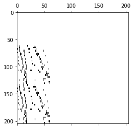
bfgrad = BilinearForm(grad(p)*w*dx).Assemble()

The matrix is still an operator on the large space!

import matplotlib.pyplot as pl
pl.spy(bfgrad.mat.ToDense())

<matplotlib.image.AxesImage at 0x7f3cf4536bf0>

Gridfunctions on product spaces consist of components

gfu = GridFunction(fes)
print("length of whole vector: ",len(gfu.vec))
gfup = gfu.components[0]
print("length of first component: ",len(gfup.vec))
gfuv = gfu.components[1]
print("length of second component: ",len(gfuv.vec))

length of whole vector:  205
length of first component:  61
length of second component:  144

Restriction and embedding operators are available:

emb_p = fes.Embedding(0)
emb_v = fes.Embedding(1)

print(emb_p.shape)
print(emb_v.shape)

res_p = fes.Restriction(0)
res_v = fes.Restriction(1)

print(res_p.shape)
print(res_v.shape)

(205, 61)
(205, 144)
(61, 205)
(144, 205)

Mixed operators

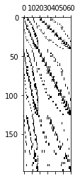
Alternatively one may define mixed operators. Note that in this case the test and trial functions must be obtained from the base spaces.

fesh1 = H1(mesh,order=order)
feshdiv = HDiv(mesh,order=order)

p_,q_ = fesh1.TnT()
v_,w_ = feshdiv.TnT()

bfgrad = BilinearForm(grad(p_)*w_*dx).Assemble()
pl.spy(bfgrad.mat.ToDense())

<matplotlib.image.AxesImage at 0x7f3cf43f6c80>

Matrices may also be transposed:

n = specialcf.normal(2)
bfdiv = BilinearForm(-div(v_)*q_*dx+v_.Trace()*n*q_*ds).Assemble()
print((bfdiv.mat.T.ToDense()-bfgrad.mat.ToDense()).Norm())

6.4456461426406835e-15