Frequency Domain: Characteristic Compactification of a Sound-Soft Circle

This notebook applies characteristic compactification to the Common circle benchmark. The characteristic construction uses the standard outgoing scaling used by conjugated infinite elements. Its coordinate is chosen so that outgoing waves reach the outer boundary along the characteristic direction, and the transformed equation contains no large \(k^2\) volume term.

We set

\[ h(r)=r, \qquad H=\frac{dh}{dr}=1. \]

The time coordinate is exactly characteristic with \(\tau=t-r\). With the convention \(e^{-ikt}\), removing \(e^{ikr}\) follows outgoing radiation along constant-\(\tau\) characteristics. The compactified outer circle is the corresponding representation of future null infinity \(\mathscr I^+\).

from ngsolve import *
from netgen.occ import *
from ngsolve.webgui import Draw
import numpy as np
from scipy.special import jv, hankel1
import matplotlib.pyplot as plt
from mpl_toolkits.axes_grid1.inset_locator import inset_axes
import ngsolve_special_functions as ng_sp
import time
notebook_start = time.perf_counter()

Characteristic compactification

Use the radial compactification

\[ \Omega(\rho)=1-\rho, \qquad r=\frac{\rho}{\Omega}=\frac{\rho}{1-\rho}, \qquad \frac12 \le \rho < 1. \]

The physical circle \(r=1\) is located at \(\rho=1/2\), and the outer boundary \(\rho=1\) represents infinity.

With the characteristic height introduced above, the exact outgoing radial amplitude and phase in two dimensions are removed by

\[ U = r^{-1/2}e^{ikr}u_{\rm char} = \left(\frac{\Omega}{\rho}\right)^{1/2}e^{ikr}u_{\rm char}. \]

Equivalently, \(u_{\rm char}=\sqrt r\,e^{-ikr}U\). We have \(u_{\rm char}=\rho^{1/2}u\). For an outgoing scattered field with asymptotics

\[ U(r,\theta) \sim r^{-1/2}e^{ikr}U_\infty(\theta), \qquad r\to\infty, \]

the transformed unknown satisfies

\[ u_{\rm char}(\rho,\theta) \to U_\infty(\theta), \qquad \rho\to1. \]

This is why the far-field pattern is simply the trace of \(u_{\rm char}\) at \(\rho=1\). The code below keeps the shorter variable names u and gfu for this characteristic unknown.

# Geometry
rho_scatterer = 0.5
rho_outer = 1.0
r_scatterer = 1.0

# Common circle-comparison target: order 8 and approximately 8,000 DOFs.
maxh = 0.140
order = 8

# Problem and reference parameters
k = 6.0
n_modes = 35

# Nominal physical mesh scale at the obstacle. Netgen's maxh is an upper bound.
dr_drho_scatterer = 1 / (1 - rho_scatterer) ** 2
nominal_kh_over_p = k * maxh * dr_drho_scatterer / order

Why the phase transformation is essential

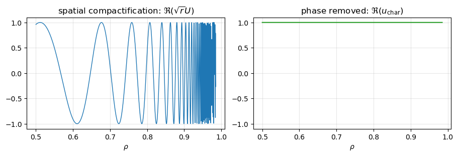
The following inexpensive one-dimensional diagnostic isolates the central numerical effect. For the prototype outgoing field \(U=r^{-1/2}e^{ikr}\), direct spatial compactification makes the phase oscillate increasingly rapidly as \(\rho\to1\). Multiplication by \(\sqrt r\) removes the radiative decay but leaves this compressed phase. The characteristic factor \(e^{-ikr}\) removes it, leaving the regular amplitude \(u_{\rm char}=1\).

rho_plot = np.linspace(rho_scatterer, 0.985, 1400)
r_plot = rho_plot / (1 - rho_plot)
outgoing = np.exp(1j * k * r_plot) / np.sqrt(r_plot)
decay_compensated = np.sqrt(r_plot) * outgoing
u_characteristic = np.exp(-1j * k * r_plot) * decay_compensated

fig, axes = plt.subplots(1, 2, figsize=(9, 3), constrained_layout=True)
axes[0].plot(rho_plot, decay_compensated.real, lw=1)
axes[0].set(title=r"spatial compactification: $\Re(\sqrt{r} U)$", xlabel=r"$\rho$")
axes[1].plot(rho_plot, u_characteristic.real, lw=1.5, color="C2")
axes[1].set(title=r"phase removed: $\Re(u_{\rm char})$", xlabel=r"$\rho$")
for ax in axes:
    ax.grid(True, alpha=0.3)
    ax.set_ylim(-1.1, 1.1)
plt.show()

With \(L=1\) and \(G=(1-\rho)^2\), the characteristic strong form of the transformed Helmholtz equation is particularly simple:

\[ \nabla\cdot\left[\left(P+GQ\right)\nabla u\right] +\left(2ik-\frac{G}{\rho}\right)n\cdot\nabla u +\frac{1}{4\rho^2}u=0, \]

where \(Q=nn^T\) is the radial projector and \(P=I-Q\) is the angular projector. The cancellation of the \(k^2\) potential is the algebraic benefit of extracting the exact outgoing phase and the spacetime consequence of following radiation along characteristics.

def create_characteristic_circle_geometry(
    rho_scatterer=rho_scatterer,
    rho_outer=rho_outer,
    draw=False,
):
    domain = Circle((0, 0), rho_outer).Face()
    domain.edges.name = "scri"
    domain.faces.name = "characteristic"

    scatterer = Circle((0, 0), rho_scatterer).Face()
    scatterer.edges.name = "scatterer"

    annulus = domain - scatterer
    annulus.faces.name = "characteristic"

    if draw:
        Draw(annulus)
    return OCCGeometry(annulus, dim=2)

geo = create_characteristic_circle_geometry(draw=True)

def solve_characteristic_circle(maxh=maxh, order=order, k=k):
    mesh = Mesh(create_characteristic_circle_geometry(draw=False).GenerateMesh(maxh=maxh))
    mesh.Curve(order + 1)

    fes = H1(mesh, order=order, complex=True, dirichlet=mesh.Boundaries("scatterer"))
    u, v = fes.TnT()

    rho = sqrt(x**2 + y**2)
    A11 = ((1 - rho) ** 2 * x**2 + y**2) / rho**2
    A12 = (-(2 - rho) * rho * x * y) / rho**2
    A22 = (x**2 + (1 - rho) ** 2 * y**2) / rho**2
    A = CF(((A11, A12), (A12, A22)), dims=(2, 2))

    B = (2j * k * rho - (1 - rho) ** 2) / rho
    Bn = CF((B * x / rho, B * y / rho))
    C = 0.25 / rho**2

    bilinear = BilinearForm(fes)
    bilinear += InnerProduct(-A * grad(u), grad(v)) * dx(bonus_intorder=8)
    bilinear += (Bn * grad(u)) * v * dx(bonus_intorder=8)
    bilinear += C * u * v * dx(bonus_intorder=8)
    bilinear.Assemble()

    theta = atan2(y, x)
    boundary_data = -np.sqrt(r_scatterer) * exp(-1j * k * r_scatterer) * exp(
        1j * k * r_scatterer * cos(theta)
    )

    gfu = GridFunction(fes)
    gfu.Set(boundary_data, definedon=mesh.Boundaries("scatterer"))

    residual = -bilinear.mat * gfu.vec
    gfu.vec.data += bilinear.mat.Inverse(freedofs=fes.FreeDofs()) * residual
    return gfu

solve_start = time.perf_counter()
gfu = solve_characteristic_circle()
solve_seconds = time.perf_counter() - solve_start
mesh = gfu.space.mesh
print(f"degrees of freedom: {gfu.space.ndof}")
print(f"ka = {k * r_scatterer:.1f}, nominal near-obstacle kh/p = {nominal_kh_over_p:.3f}")
print(f"mesh, assembly, and direct solve: {solve_seconds:.3f} s")

degrees of freedom: 8300
ka = 6.0, nominal near-obstacle kh/p = 0.420
mesh, assembly, and direct solve: 0.224 s

Far-field reference

The common Fourier–Bessel reference is given in Common circle benchmark. Since the characteristic unknown already removes \(r^{-1/2}e^{ikr}\), this notebook extracts the numerical far field as

\[ U_{\infty,h}(\theta)=u_h(\rho=1,\theta). \]

def far_field_cf(k=k, N=n_modes):
    rho = sqrt(x**2 + y**2)
    nx = x / rho
    ny = y / rho

    cf = -ng_sp.jv(k, 0) / ng_sp.hankel1(k, 0)
    for n in range(1, N + 1):
        angular = (nx + 1j * ny) ** n + (nx - 1j * ny) ** n
        cf -= angular * ng_sp.jv(k, n) / ng_sp.hankel1(k, n)

    return np.sqrt(2 / (np.pi * k)) * np.exp(-1j * np.pi / 4) * cf


def far_field_pattern(thetas, k=k, N=n_modes):
    thetas = np.asarray(thetas, dtype=float)
    n = np.arange(-N, N + 1)
    coefficients = -jv(n, k) / hankel1(n, k)
    return np.sqrt(2 / (np.pi * k)) * np.exp(-1j * np.pi / 4) * (
        coefficients @ np.exp(1j * np.outer(n, thetas))
    )


def far_field_l2_error(gfu, reference_ff):
    mesh = gfu.space.mesh
    difference = gfu - reference_ff
    err_sq = Integrate(difference * Conj(difference), mesh, definedon=mesh.Boundaries("scri")).real
    norm_sq = Integrate(reference_ff * Conj(reference_ff), mesh, definedon=mesh.Boundaries("scri")).real
    return np.sqrt(err_sq / norm_sq)


def sample_far_field(gfu, thetas, eps=1e-8):
    sample_radius = 1 - eps
    return np.array(
        [gfu(sample_radius * np.cos(theta), sample_radius * np.sin(theta)) for theta in thetas],
        dtype=complex,
    )

reference_start = time.perf_counter()
reference_far_field = far_field_cf()
far_field_rel_error = far_field_l2_error(gfu, reference_far_field)
reference_seconds = time.perf_counter() - reference_start
print(f"relative far-field L2 error at scri: {far_field_rel_error:.3e}")
print(f"analytic reference evaluation: {reference_seconds:.3f} s")

relative far-field L2 error at scri: 4.055e-08
analytic reference evaluation: 0.091 s

Far-field angular distribution

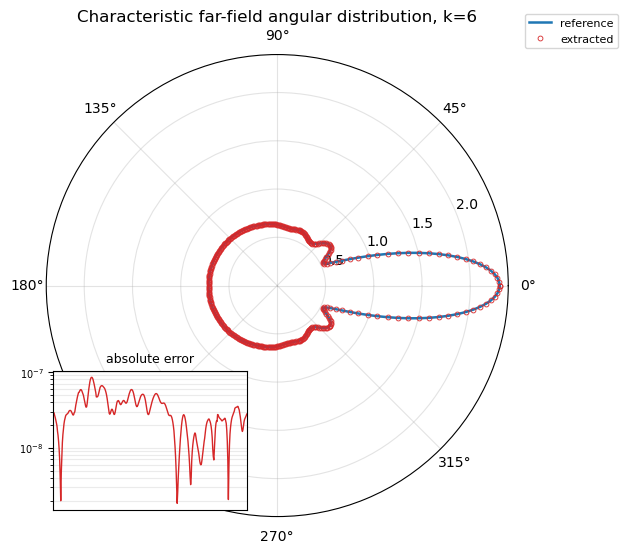
The polar plot shows the angular distribution of the far field. The inset shows the absolute error against the analytic Fourier-Bessel reference.

thetas = np.linspace(0, 2 * np.pi, 361, endpoint=True)
ff_num = sample_far_field(gfu, thetas)
ff_ref = far_field_pattern(thetas)
absolute_error = np.abs(ff_num - ff_ref)

fig = plt.figure(figsize=(6, 6))
ax = fig.add_subplot(111, projection="polar")

ax.plot(thetas, np.abs(ff_ref), color="C0", lw=1.8, label="reference")
ax.plot(
    thetas,
    np.abs(ff_num),
    linestyle="None",
    marker="o",
    markerfacecolor="none",
    markersize=3.5,
    markeredgewidth=0.6,
    color="C3",
    label="extracted",
)
ax.set_title(f"Characteristic far-field angular distribution, k={k:g}", pad=24)
ax.grid(True, alpha=0.35)
ax.legend(loc="upper right", bbox_to_anchor=(1.25, 1.10), fontsize=8)

axins = inset_axes(ax, width="42%", height="30%", loc="lower left")
axins.semilogy(thetas, np.maximum(absolute_error, 1e-16), color="C3", lw=1)
axins.set_title("absolute error", fontsize=9)
axins.set_xlim(0, 2 * np.pi)
axins.set_xticks([])
axins.tick_params(axis="y", labelsize=7)
axins.grid(True, which="both", alpha=0.25)

plt.show()

Compactified solution

The solution shown below is the characteristic unknown u. Unlike the original scattered field variable, it is nonoscillatory and finite at the compactified boundary.

Draw(gfu, mesh, "characteristic compactified scattered field", min=-1, max=1)
print(f"notebook compute time after imports: {time.perf_counter() - notebook_start:.3f} s")

notebook compute time after imports: 0.871 s

Remarks

• The characteristic choice H=1 matches the outgoing phase everywhere, not only near infinity.

• In spacetime language, the method follows outgoing radiation along retarded-time characteristics toward future null infinity.

• In frequency-domain language, the same choice removes the leading factor r^(-1/2) exp(i k r) before discretization.