Explicit DG for the Trapping Square

This notebook develops the time-domain discretization from scratch with explicit evolution as the design goal. Three DG routes were screened on the same mesh:

formulation	persistent state in 2D	dominant spectral radius	main drawback
primal SIPDG, aggressively tuned penalty	\(2N\)	\(\approx 977\)	penalty controls the CFL limit
characteristic-upwind symmetric system	\(3N\)	\(\approx 624\)	denser and deliberately dissipative
central factor DG, auxiliary field eliminated	\(2N\)	\(\approx 408\)	requires an exact local vector-mass inverse

The measurements above use \(p=3\) and maxh=0.20; they are a formulation screen, not universal constants. The last option is both the fastest here and the cleanest for a trapping calculation: it has a discrete energy identity, no SIP penalty, and no interior upwind damping to contaminate the ringdown. We use a finer default mesh below and determine its actual RK4 step from its spectrum.

from ngsolve import *
from netgen.occ import *
from ngsolve.webgui import Draw
import ngsolve as ng

import matplotlib.pyplot as plt
import numpy as np
from scipy import sparse
from scipy.sparse.linalg import LinearOperator, eigs, eigsh, norm as sparse_norm, splu
import time

notebook_start = time.perf_counter()

Geometry, resolution, and drive

The physical geometry and source frequency are unchanged. Polynomial degree three with maxh=0.15 gives the nominal physical-region resolution \(\omega h/p=0.54\). The drive is smoothly windowed to zero: an abrupt cutoff would inject broadband energy precisely into the modes that determine an explicit CFL limit.

In the layer we use

\[ \Omega(s)=1-2s^2+s^3, \qquad s=\frac{\rho-R}{R_{\rm out}-R}. \]

It has \(\Omega=1\) and \(\Omega'=0\) at the layer interface and the same linear zero as the usual profile at null infinity. Thus the coordinate coefficients join the physical region continuously without increasing the measured CFL cost.

# Geometry
Rout = 2.0
RScat = 1.0
DScat = 0.1
DHole = 0.2
R = 1.5
xOffset = 0.5

# Space and time
maxh = 0.15
order = 3
drive_frequency = 10.8
drive_until = 3.0
t_end = 6.0
source_amplitude = 100.0
source_ramp = 0.5
cfl_safety = 0.80


def create_trapping_geometry():
    domain = Circle((0, 0), Rout).Face()
    domain.edges.name = "outer"
    domain.faces.name = "outer"

    inner = Circle((0, 0), R).Face()
    inner.edges.name = "interface"
    inner.faces.name = "inner"

    wall = (
        MoveTo(-RScat / 2 + xOffset, -RScat / 2).Rectangle(RScat, RScat).Face()
        - MoveTo(-RScat / 2 + DScat / 2 + xOffset, -RScat / 2 + DScat / 2)
          .Rectangle(RScat - DScat, RScat - DScat).Face()
        - MoveTo(-RScat / 2 - DScat + xOffset, -DHole / 2)
          .Rectangle(2 * DScat, DHole).Face()
    )
    wall.edges.name = "scatterer"

    cavity = (
        MoveTo(-RScat / 2 + xOffset, -RScat / 2).Rectangle(RScat, RScat).Face()
        - wall
    )
    cavity.faces.name = "cavity"

    return OCCGeometry(Glue([domain - inner, inner - cavity - wall, cavity]), dim=2)


mesh = Mesh(create_trapping_geometry().GenerateMesh(maxh=maxh))
mesh.Curve(order)
Vp = L2(mesh, order=order, dgjumps=True)
Vz = VectorL2(mesh, order=order, dgjumps=True)

Draw(mesh)
print(f"elements: {mesh.ne}")
print(f"scalar DG degrees of freedom: {Vp.ndof}")
print(f"nominal physical-region omega h/p: {drive_frequency * maxh / order:.3f}")

elements: 1181
scalar DG degrees of freedom: 11810
nominal physical-region omega h/p: 0.540

Symmetric factorization of the continuous operator

Write \(e_r=X/\rho\), \(Q=e_re_r^T\), \(P=I-Q\), and \(A=GQ+LP\). Define

\[ S=A^{1/2}=\frac{\Omega}{\sqrt L}Q+\sqrt L P, \qquad d=\frac{\Omega'}{2\sqrt L}e_r, \qquad \mathcal D u=S\nabla u+d u. \]

Then \(S^TS=A\), \(S^Td=g\), and \(d\cdot d=(\Omega')^2/(4L)\), so the entire conformal spatial volume form factors exactly:

\[ K(u,v)=(\mathcal D u,\mathcal D v). \]

Moreover, \(S\mathcal D u=A\nabla u+g u\) is the full conformal flux. Introducing \(p=u_t\) and \(z=\mathcal D u\) gives a symmetric-hyperbolic principal system whose normal matrix is

\[\begin{split} \mathcal A_n= \begin{pmatrix}2b\cdot n&-(Sn)^T\\-Sn&0\end{pmatrix}, \qquad b=He_r. \end{split}\]

At null infinity \(Sn=0\), \(m=1+H=2\), and \(b\cdot n=1\), so its speeds are \(1,0,0\): there is no incoming characteristic and no outer boundary condition.

rho = sqrt(ng.x**2 + ng.y**2)
radial = CF((ng.x, ng.y))
er = radial / rho
Q = OuterProduct(er, er)
P = Id(2) - Q

s = (rho - R) / (Rout - R)
Omega = mesh.MaterialCF({"outer": 1 - 2 * s**2 + s**3}, default=1)
DOmega = Omega.Diff(rho)
L = Omega - rho * DOmega
G = Omega**2 / L
H = mesh.MaterialCF({"outer": 1 - G}, default=0)

mass_weight = 1 + H
transport_vector = H * er
S = Omega / sqrt(L) * Q + sqrt(L) * P
d = DOmega / (2 * sqrt(L)) * er

Central DG derivative and the mixed transport term

Let \(V_h=L^2_p\) and \(Z_h=[L^2_p]^2\). The central discrete conformal derivative \(B:V_h\to Z_h'\) is

\[ \begin{aligned} (Bu,w)={}&\sum_K(\mathcal D u,w)_K -\sum_F [u]\,\{Sw\}\cdot n -\int_{\Gamma_{\rm wall}}u\,Sw\cdot n. \end{aligned} \]

Thus \(u^*=\{u\}\) on interior faces and \(u^*=0\) at the sound-soft wall. There is no term at null infinity because \(Sn=0\). Using the exact algebraic transpose \(B^T\) makes the two first-order equations an adjoint pair.

The mixed time-space operator must be paired just as carefully. Its volume and skeleton terms are skew, leaving only the physical outflow:

\[ C_h(v,v)=\int_{\mathscr I^+}v^2\,ds. \]

In particular, the \(B^T\) and \(C_h\) face contributions combine into the correct interface flux \((Sz-bp)\cdot n\).

u, v = Vp.TnT()
z, w = Vz.TnT()
normal = specialcf.normal(mesh.dim)

mass_p_form = mass_weight * u * v * dx
mass_z_form = InnerProduct(z, w) * dx

average_transport = 0.5 * (transport_vector + transport_vector.Other())
transport_form = (
    -u * InnerProduct(transport_vector, grad(v)) * dx
    + v * InnerProduct(transport_vector, grad(u)) * dx
    + InnerProduct(average_transport, normal)
      * (u.Other() * v - u * v.Other()) * dx(skeleton=True)
    + u * v * ds("outer", skeleton=True)
)

trial_u = Vp.TrialFunction()
test_z = Vz.TestFunction()
jump_u = trial_u - trial_u.Other()
average_S_test = S * test_z + S.Other() * test_z.Other()

derivative_form = (
    InnerProduct(S * grad(trial_u) + d * trial_u, test_z) * dx
    - 0.5 * jump_u * InnerProduct(average_S_test, normal) * dx(skeleton=True)
    - trial_u * InnerProduct(S * test_z, normal)
      * ds("scatterer", skeleton=True)
)

Exact local elimination and the penalty-free stiffness

The semidiscrete first-order pair is

\[ M_p\dot p+Cp+B^Tz=f, \qquad M_z\dot z-Bp=0. \]

Compatible data preserve \(z=M_z^{-1}Bu\). We therefore eliminate \(z\) and evolve only two scalar states,

\[ \dot u=p, \qquad M_p\dot p=f-Cp-K_hu, \qquad K_h=B^TM_z^{-1}B. \]

This is a central LDG/BR factorization, not SIPDG. It needs no penalty because \(K_h\) is positive by construction. Both mass inverses below consist of disjoint element blocks. Specifying blocktype="element" is essential for VectorL2; its default smoothing blocks overlap. We materialize \(K_h\) once because an assembled sparse product is substantially faster on this CPU problem than applying its three factors at every RK stage.

setup_start = time.perf_counter()

Mp = BilinearForm(mass_p_form).Assemble().mat
Mz = BilinearForm(mass_z_form).Assemble().mat
C = BilinearForm(transport_form).Assemble().mat

B_form = BilinearForm(Vp, Vz)
B_form += derivative_form
B = B_form.Assemble().mat
BT = B.T.CreateSparseMatrix()

blocks_p = Vp.CreateSmoothingBlocks(blocktype="element")
blocks_z = Vz.CreateSmoothingBlocks(blocktype="element")
Mp_inverse = Mp.CreateBlockSmoother(blocks_p, parallel=True)
Mz_inverse = Mz.CreateBlockSmoother(blocks_z, parallel=True)

K = (BT @ Mz_inverse @ B).CreateSparseMatrix()
outer_flux = BilinearForm(
    u * v * ds("outer", skeleton=True), check_unused=False
).Assemble().mat

setup_seconds = time.perf_counter() - setup_start
print(f"operator setup: {setup_seconds:.3f} s")
print(f"materialized K nonzeros: {K.nze}")

operator setup: 0.740 s
materialized K nonzeros: 1112100

Algebraic energy audits

These checks target failure modes that a single quadratic probe cannot see:

\[ C+C^T=2B_{\mathscr I^+}, \qquad K=K^T, \qquad K=B^TM_z^{-1}B. \]

We also verify both local mass inverses and the semidiscrete energy law

\[ E_h=\frac12\left(p^TM_pp+u^TKu\right), \qquad \dot E_h=p^Tf-p^TB_{\mathscr I^+}p. \]

def scipy_csr(matrix):
    result = sparse.csr_matrix(matrix.CSR()).copy()
    result.sum_duplicates()
    result.eliminate_zeros()
    return result


def local_inverse_residual(matrix, inverse, rng):
    rhs = matrix.CreateVector()
    rhs.FV().NumPy()[:] = rng.standard_normal(matrix.height)
    solution = rhs.CreateVector()
    inverse.Mult(rhs, solution)
    residual = rhs.CreateVector()
    matrix.Mult(solution, residual)
    residual.data -= rhs
    return Norm(residual) / Norm(rhs)


rng = np.random.default_rng(12)
Mp_sparse = scipy_csr(Mp)
Mz_sparse = scipy_csr(Mz)
C_sparse = scipy_csr(C)
B_sparse = scipy_csr(B)
K_sparse = scipy_csr(K)
outer_sparse = scipy_csr(outer_flux)

mass_p_residual = local_inverse_residual(Mp, Mp_inverse, rng)
mass_z_residual = local_inverse_residual(Mz, Mz_inverse, rng)
mass_p_symmetry = sparse_norm(Mp_sparse - Mp_sparse.T) / sparse_norm(Mp_sparse)
mass_z_symmetry = sparse_norm(Mz_sparse - Mz_sparse.T) / sparse_norm(Mz_sparse)
stiffness_symmetry = sparse_norm(K_sparse - K_sparse.T) / sparse_norm(K_sparse)
transport_identity = (
    sparse_norm(C_sparse + C_sparse.T - 2 * outer_sparse)
    / sparse_norm(2 * outer_sparse)
)

probe_u = GridFunction(Vp).vec
probe_z = GridFunction(Vz).vec
probe_u.FV().NumPy()[:] = rng.standard_normal(Vp.ndof)
probe_z.FV().NumPy()[:] = rng.standard_normal(Vz.ndof)

B_probe = probe_z.CreateVector()
BT_probe = probe_u.CreateVector()
B.Mult(probe_u, B_probe)
BT.Mult(probe_z, BT_probe)
transpose_residual = abs(
    probe_z.InnerProduct(B_probe) - probe_u.InnerProduct(BT_probe)
) / max(abs(probe_z.InnerProduct(B_probe)), 1.0)

flux_probe = probe_z.CreateVector()
Mz_inverse.Mult(B_probe, flux_probe)
factored_K_probe = probe_u.CreateVector()
materialized_K_probe = probe_u.CreateVector()
BT.Mult(flux_probe, factored_K_probe)
K.Mult(probe_u, materialized_K_probe)
factored_K_probe.data -= materialized_K_probe
factorization_residual = Norm(factored_K_probe) / Norm(materialized_K_probe)

probe_p = probe_u.CreateVector()
probe_p.FV().NumPy()[:] = rng.standard_normal(Vp.ndof)
C_probe = probe_p.CreateVector()
K_probe = probe_u.CreateVector()
dual_rhs = probe_p.CreateVector()
probe_pdot = probe_p.CreateVector()
C.Mult(probe_p, C_probe)
K.Mult(probe_u, K_probe)
dual_rhs.data = -C_probe
dual_rhs.data -= K_probe
Mp_inverse.Mult(dual_rhs, probe_pdot)
energy_derivative = (
    probe_p.InnerProduct(Mp * probe_pdot)
    + probe_p.InnerProduct(K_probe)
).real
outflow_derivative = -probe_p.InnerProduct(outer_flux * probe_p).real
energy_identity_residual = abs(energy_derivative - outflow_derivative) / max(
    abs(outflow_derivative), 1.0
)

print(f"scalar local-mass residual: {mass_p_residual:.3e}")
print(f"vector local-mass residual: {mass_z_residual:.3e}")
print(f"M_p / M_z symmetry: {mass_p_symmetry:.3e} / {mass_z_symmetry:.3e}")
print(f"K symmetry: {stiffness_symmetry:.3e}")
print(f"C+C^T=2 B_scri residual: {transport_identity:.3e}")
print(f"B transpose polarization residual: {transpose_residual:.3e}")
print(f"materialized-factorized K residual: {factorization_residual:.3e}")
print(f"semidiscrete energy residual: {energy_identity_residual:.3e}")

assert mass_p_residual < 1e-11 and mass_z_residual < 1e-11
assert max(mass_p_symmetry, mass_z_symmetry, stiffness_symmetry) < 1e-12
assert transport_identity < 1e-12
assert transpose_residual < 1e-12
assert factorization_residual < 1e-12
assert energy_identity_residual < 1e-11

scalar local-mass residual: 1.841e-16
vector local-mass residual: 1.674e-16
M_p / M_z symmetry: 0.000e+00 / 0.000e+00
K symmetry: 1.964e-16
C+C^T=2 B_scri residual: 2.421e-16
B transpose polarization residual: 1.851e-16
materialized-factorized K residual: 5.048e-16
semidiscrete energy residual: 1.763e-14

Spectrum-based RK4 step

Classical RK4 is slightly more efficient per operator evaluation than the common five-stage low-storage RK method for this nearly imaginary spectrum. We estimate the spectral radius of the actual first-order state generator

\[\begin{split} \mathcal A_h \begin{pmatrix}u\\p\end{pmatrix} = \begin{pmatrix} p\\-M_p^{-1}(Ku+Cp) \end{pmatrix}, \end{split}\]

rather than relying on a mesh-only CFL formula. RK4 reaches \(2\sqrt2\) on the imaginary axis; we retain a 20% margin and shorten the step slightly so that the source switches off exactly at a step boundary.

cfl_start = time.perf_counter()

# The four eigenvalues closest to zero also audit the central derivative for a
# scalar checkerboard kernel. Their positivity is not a mesh-independent proof,
# but no collapsing mode was observed in the h=0.25, 0.20, 0.15 refinement audit.
low_stiffness_eigenvalues = np.sort(
    eigsh(
        K_sparse,
        k=4,
        M=Mp_sparse,
        sigma=0.0,
        which="LM",
        return_eigenvectors=False,
        tol=1e-7,
    )
)

Mp_lu = splu(Mp_sparse.tocsc())  # used only by the spectral estimator


def apply_state_generator(state):
    displacement = state[: Vp.ndof]
    velocity = state[Vp.ndof :]
    acceleration = Mp_lu.solve(
        -K_sparse @ displacement - C_sparse @ velocity
    )
    return np.concatenate((velocity, acceleration))


state_operator = LinearOperator(
    (2 * Vp.ndof, 2 * Vp.ndof),
    matvec=apply_state_generator,
    dtype=float,
)
dominant_eigenvalues = eigs(
    state_operator,
    k=10,
    which="LM",
    return_eigenvectors=False,
    v0=rng.standard_normal(2 * Vp.ndof),
    tol=2e-5,
    maxiter=2000,
    ncv=36,
)
spectral_radius = float(np.max(np.abs(dominant_eigenvalues)))

rk4_imaginary_radius = 2 * np.sqrt(2)
raw_dt = cfl_safety * rk4_imaginary_radius / spectral_radius
steps_to_switch_off = int(np.ceil(drive_until / raw_dt))
dt = drive_until / steps_to_switch_off
nsteps = int(round(t_end / dt))
assert abs(nsteps * dt - t_end) < 1e-12


def rk4_polynomial(z):
    return 1 + z + z**2 / 2 + z**3 / 6 + z**4 / 24


sampled_amplification = float(
    np.max(np.abs(rk4_polynomial(dt * dominant_eigenvalues)))
)
cfl_seconds = time.perf_counter() - cfl_start

print(f"low generalized K eigenvalues: {low_stiffness_eigenvalues}")
print(f"state spectral radius: {spectral_radius:.6f}")
print(f"raw CFL step / selected step: {raw_dt:.8f} / {dt:.8f}")
print(f"RK4 steps: {nsteps} ({steps_to_switch_off} to source-off)")
print(f"largest sampled RK4 amplification: {sampled_amplification:.6f}")
print(f"spectral audit: {cfl_seconds:.3f} s")

assert low_stiffness_eigenvalues[0] > 0
assert sampled_amplification <= 1 + 1e-5

low generalized K eigenvalues: [0.08078045 0.47650098 0.65418386 0.65740427]
state spectral radius: 386.610456
raw CFL step / selected step: 0.00585277 / 0.00584795
RK4 steps: 1026 (513 to source-off)
largest sampled RK4 amplification: 0.716255
spectral audit: 3.654 s

Smooth source and explicit RK4 kernel

The nonic smoothstep below has four vanishing derivatives at both endpoints. It ramps the sinusoid on and off without a high-frequency cutoff impulse. Every RK stage evaluates the source at its own stage time. The production loop uses one sparse \(K\) product, one sparse \(C\) product, and one exact element-local scalar mass inverse per stage—there is no global solve.

source_profile = exp(-30 * ((ng.x + 0.8) ** 2 + (ng.y + 0.8) ** 2))
force = LinearForm(
    source_amplitude * source_profile * Vp.TestFunction() * dx("inner|cavity")
).Assemble().vec


def nonic_smoothstep(value):
    value = np.clip(value, 0.0, 1.0)
    return value**5 * (
        126 + value * (-420 + value * (540 + value * (-315 + 70 * value)))
    )


def drive_amplitude(t):
    if t <= 0.0 or t >= drive_until:
        return 0.0
    if t < source_ramp:
        envelope = nonic_smoothstep(t / source_ramp)
    elif t > drive_until - source_ramp:
        envelope = nonic_smoothstep((drive_until - t) / source_ramp)
    else:
        envelope = 1.0
    return float(envelope * np.sin(drive_frequency * t))


def make_rk4_workspace(template):
    return {
        "u0": template.CreateVector(),
        "p0": template.CreateVector(),
        "stage_u": template.CreateVector(),
        "stage_p": template.CreateVector(),
        "k_u": [template.CreateVector() for _ in range(4)],
        "k_p": [template.CreateVector() for _ in range(4)],
        "C_p": template.CreateVector(),
        "K_u": template.CreateVector(),
        "dual_rhs": template.CreateVector(),
    }


rk_stage_offsets = (0.0, 0.5, 0.5, 1.0)
rk_stage_times = (0.0, 0.5, 0.5, 1.0)
rk_weights = (1 / 6, 1 / 3, 1 / 3, 1 / 6)


def rk4_step(displacement, velocity, t, step, workspace, amplitude_function):
    u0 = workspace["u0"]
    p0 = workspace["p0"]
    stage_u = workspace["stage_u"]
    stage_p = workspace["stage_p"]
    k_u = workspace["k_u"]
    k_p = workspace["k_p"]
    C_p = workspace["C_p"]
    K_u = workspace["K_u"]
    dual_rhs = workspace["dual_rhs"]

    u0.data = displacement
    p0.data = velocity
    source_power = 0.0
    outflow_power = 0.0

    for stage, (offset, stage_time, weight) in enumerate(
        zip(rk_stage_offsets, rk_stage_times, rk_weights)
    ):
        stage_u.data = u0
        stage_p.data = p0
        if stage:
            stage_u.data += offset * step * k_u[stage - 1]
            stage_p.data += offset * step * k_p[stage - 1]

        k_u[stage].data = stage_p
        C.Mult(stage_p, C_p)
        K.Mult(stage_u, K_u)
        dual_rhs.data = -C_p
        dual_rhs.data -= K_u

        amplitude = amplitude_function(t + stage_time * step)
        if amplitude:
            dual_rhs.data += amplitude * force
        Mp_inverse.Mult(dual_rhs, k_p[stage])

        source_power += weight * amplitude * stage_p.InnerProduct(force).real
        outflow_power += weight * stage_p.InnerProduct(C_p).real

    displacement.data = u0
    velocity.data = p0
    for weight, derivative_u, derivative_p in zip(rk_weights, k_u, k_p):
        displacement.data += step * weight * derivative_u
        velocity.data += step * weight * derivative_p

    return step * source_power, step * outflow_power


def discrete_energy(displacement, velocity, K_work=None):
    if K_work is None:
        K_work = displacement.CreateVector()
    K.Mult(displacement, K_work)
    return 0.5 * (
        velocity.InnerProduct(Mp * velocity) + displacement.InnerProduct(K_work)
    ).real

High-frequency stability stress test

A random discontinuous displacement and velocity excite the top of the DG spectrum. We normalize their energy to one and evolve them without a source. At the selected step RK4 must remain finite and must not produce energy growth.

stress_u = GridFunction(Vp, name="stress_u")
stress_p = GridFunction(Vp, name="stress_p")
stress_u.vec.FV().NumPy()[:] = rng.standard_normal(Vp.ndof)
stress_p.vec.FV().NumPy()[:] = rng.standard_normal(Vp.ndof)

stress_initial_energy = discrete_energy(stress_u.vec, stress_p.vec)
stress_scale = 1 / np.sqrt(stress_initial_energy)
stress_u.vec.data *= stress_scale
stress_p.vec.data *= stress_scale

stress_workspace = make_rk4_workspace(stress_u.vec)
stress_energies = [discrete_energy(stress_u.vec, stress_p.vec)]
zero_drive = lambda t: 0.0
stress_steps = 120

with TaskManager():
    for stress_step in range(stress_steps):
        rk4_step(
            stress_u.vec,
            stress_p.vec,
            stress_step * dt,
            dt,
            stress_workspace,
            zero_drive,
        )
        stress_energies.append(discrete_energy(stress_u.vec, stress_p.vec))

stress_energies = np.asarray(stress_energies)
stress_growth = np.max(stress_energies) / stress_energies[0] - 1
print(f"random high-frequency stress growth: {stress_growth:.3e}")
print(f"stress final/initial energy: {stress_energies[-1] / stress_energies[0]:.6f}")

assert np.all(np.isfinite(stress_energies))
assert stress_growth < 1e-6

random high-frequency stress growth: 0.000e+00
stress final/initial energy: 0.525081

Driven evolution, energy balance, and trapping diagnostics

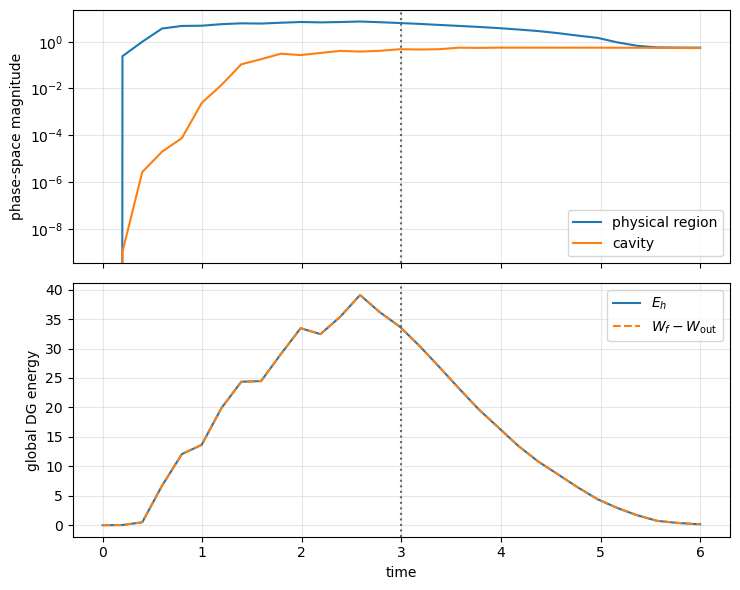
The global DG energy is the stability diagnostic. In the unchanged physical region, \(S=I\) and \(d=0\), so the eliminated vector \(z=M_z^{-1}Bu\) is the DG gradient. We use it to measure \(\bigl(\|p\|^2+\|z\|^2\bigr)^{1/2}\) in the physical region and cavity. Source work and null-infinity outflow are accumulated with the RK4 stage weights, allowing a direct audit of

\[ E_h(t)-E_h(0)-W_f(t)+W_{\mathscr I^+}(t)=0. \]

z_trial, z_test = Vz.TnT()
physical_p_mass = BilinearForm(
    u * v * dx("inner|cavity"), check_unused=False
).Assemble().mat
cavity_p_mass = BilinearForm(
    u * v * dx("cavity"), check_unused=False
).Assemble().mat
physical_z_mass = BilinearForm(
    InnerProduct(z_trial, z_test) * dx("inner|cavity"), check_unused=False
).Assemble().mat
cavity_z_mass = BilinearForm(
    InnerProduct(z_trial, z_test) * dx("cavity"), check_unused=False
).Assemble().mat


def recovered_flux(displacement, dual_work, flux_work):
    B.Mult(displacement, dual_work)
    Mz_inverse.Mult(dual_work, flux_work)


def phase_space_magnitudes(velocity, flux):
    physical_sq = (
        velocity.InnerProduct(physical_p_mass * velocity)
        + flux.InnerProduct(physical_z_mass * flux)
    ).real
    cavity_sq = (
        velocity.InnerProduct(cavity_p_mass * velocity)
        + flux.InnerProduct(cavity_z_mass * flux)
    ).real
    return np.sqrt(max(physical_sq, 0.0)), np.sqrt(max(cavity_sq, 0.0))


def run_simulation():
    displacement = GridFunction(Vp, name="u_explicit_dg")
    velocity = GridFunction(Vp, name="ut_explicit_dg")
    animation = GridFunction(Vp, multidim=0, name="explicit_dg_history")
    workspace = make_rk4_workspace(displacement.vec)

    dual_flux = GridFunction(Vz).vec
    flux = GridFunction(Vz, name="conformal_gradient").vec
    energy_work = displacement.vec.CreateVector()

    diagnostic_stride = max(1, int(round(0.2 / dt)))
    frame_stride = max(1, int(round(0.5 / dt)))
    progress_stride = max(1, int(round(1.0 / dt)))

    times = []
    energies = []
    source_work = []
    outflow = []
    physical_magnitudes = []
    cavity_magnitudes = []
    cumulative_work = 0.0
    cumulative_outflow = 0.0

    def record(t):
        recovered_flux(displacement.vec, dual_flux, flux)
        physical, cavity = phase_space_magnitudes(velocity.vec, flux)
        times.append(t)
        energies.append(discrete_energy(displacement.vec, velocity.vec, energy_work))
        source_work.append(cumulative_work)
        outflow.append(cumulative_outflow)
        physical_magnitudes.append(physical)
        cavity_magnitudes.append(cavity)

    record(0.0)
    animation.AddMultiDimComponent(displacement.vec)

    evolution_start = time.perf_counter()
    with TaskManager():
        for step_index in range(nsteps):
            t = step_index * dt
            work_increment, outflow_increment = rk4_step(
                displacement.vec,
                velocity.vec,
                t,
                dt,
                workspace,
                drive_amplitude,
            )
            cumulative_work += work_increment
            cumulative_outflow += outflow_increment

            completed_step = step_index + 1
            if completed_step % diagnostic_stride == 0 or completed_step == nsteps:
                record(completed_step * dt)
            if completed_step % frame_stride == 0:
                animation.AddMultiDimComponent(displacement.vec)
            if completed_step % progress_stride == 0:
                print(f"t={completed_step * dt:5.2f}", end="\r")

    if nsteps % frame_stride:
        animation.AddMultiDimComponent(displacement.vec)
    evolution_seconds = time.perf_counter() - evolution_start
    print(f"t={t_end:5.2f}")

    return {
        "displacement": displacement,
        "velocity": velocity,
        "animation": animation,
        "times": np.asarray(times),
        "energies": np.asarray(energies),
        "source_work": np.asarray(source_work),
        "outflow": np.asarray(outflow),
        "physical": np.asarray(physical_magnitudes),
        "cavity": np.asarray(cavity_magnitudes),
        "seconds": evolution_seconds,
    }


result = run_simulation()

t= 1.00

t= 2.00

t= 3.00

t= 4.00

t= 5.00

t= 6.00
t= 6.00

energy_balance = (
    result["energies"]
    - result["energies"][0]
    - result["source_work"]
    + result["outflow"]
)
balance_scale = max(
    np.max(np.abs(result["energies"])),
    np.max(np.abs(result["source_work"])),
    np.max(np.abs(result["outflow"])),
    1.0,
)
relative_energy_balance = np.max(np.abs(energy_balance)) / balance_scale

post_drive = result["times"] >= drive_until - 0.5 * dt
post_drive_energy = result["energies"][post_drive]
post_drive_increase = max(0.0, np.max(np.diff(post_drive_energy), initial=0.0))
post_drive_increase /= max(np.max(post_drive_energy), 1.0)

all_histories = np.concatenate(
    [
        result["energies"],
        result["source_work"],
        result["outflow"],
        result["physical"],
        result["cavity"],
    ]
)
rhs_evaluations = 4 * nsteps
million_dof_stage_updates = (
    rhs_evaluations * 2 * Vp.ndof / result["seconds"] / 1e6
)

print(f"RK4 evolution: {result['seconds']:.3f} s")
print(f"RHS evaluations per second: {rhs_evaluations / result['seconds']:.1f}")
print(f"million scalar-state stage updates/s: {million_dof_stage_updates:.2f}")
print(f"maximum normalized energy-balance residual: {relative_energy_balance:.3e}")
print(f"post-drive sampled energy increase: {post_drive_increase:.3e}")

assert np.all(np.isfinite(all_histories))
assert np.all(np.isfinite(result["displacement"].vec.FV().NumPy()))
assert np.all(np.isfinite(result["velocity"].vec.FV().NumPy()))
assert relative_energy_balance < 1e-4
assert post_drive_increase < 1e-4

RK4 evolution: 2.378 s
RHS evaluations per second: 1725.8
million scalar-state stage updates/s: 40.76
maximum normalized energy-balance residual: 7.218e-08
post-drive sampled energy increase: 0.000e+00

Draw(
    result["animation"],
    mesh,
    "explicit penalty-free DG evolution",
    min=-0.1,
    max=0.1,
    animate=True,
)

fig, axes = plt.subplots(2, 1, figsize=(7.5, 6), sharex=True)

axes[0].semilogy(result["times"], result["physical"], label="physical region")
axes[0].semilogy(result["times"], result["cavity"], label="cavity")
axes[0].set_ylabel("phase-space magnitude")
axes[0].legend()

axes[1].plot(result["times"], result["energies"], label="$E_h$")
axes[1].plot(
    result["times"],
    result["source_work"] - result["outflow"],
    "--",
    label="$W_f-W_{\\mathrm{out}}$",
)
axes[1].set(xlabel="time", ylabel="global DG energy")
axes[1].legend()

for axis in axes:
    axis.axvline(drive_until, color="0.4", ls=":", label="source off")
    axis.grid(True, which="both", alpha=0.3)

plt.tight_layout()
plt.show()

print(f"notebook compute time after imports: {time.perf_counter() - notebook_start:.3f} s")

notebook compute time after imports: 8.034 s

Interpretation and implementation choice

The source-work/outflow curve lies on top of the discrete energy, while the source-free stress test shows no high-frequency growth. These are stronger stability checks than simply observing a bounded animation. After the drive ends, radiation crosses null infinity and the global energy falls; the cavity curve isolates the slower trapped component.

The decisive formulation choice is the adjoint factorization \(K_h=B^TM_z^{-1}B\). A primal SIP form carries fewer temporary vector unknowns, but its penalty creates much faster eigenmodes and therefore many more explicit steps. A fully characteristic-upwind symmetric system removes the penalty too, but carries three dynamic fields, has a denser operator, and adds jump dissipation that is undesirable when measuring a weakly damped resonance. The central factor method retains the symmetric-hyperbolic energy structure, eliminates the auxiliary field, and introduces no artificial interior damping.

For this assembled CPU implementation, materializing \(K_h\) is fastest. At much higher order or on accelerators, applying \(B\), the local vector mass inverse, and \(B^T\) matrix-free may become preferable. Either implementation remains explicit: the only inverse used during evolution is the exact, independent scalar mass block on each element.