Frequency Domain: Poincaré Compactification of a Sound-Soft Circle

This notebook has a particularly fun example: the Poincaré compactification maps the exterior of the Common circle benchmark to a hyperbolic disk. The same conformal geometry that represents an infinite hyperbolic plane inside a finite disk also helps solve the Helmholtz equation numerically on the unbounded domain.

From the hyperboloid to the Poincaré disk

Start with \((2+1)\)-dimensional Minkowski spacetime in polar coordinates,

\[ ds^2_{\mathbb M} = -dt^2 + dr^2 + r^2 d\theta^2. \]

As demonstrated by Minkowski in his 1908 lecture, the unit hyperboloid is the Lorentzian analogue of the unit sphere in Euclidean space. The surface

\[ t^2-r^2=1, \qquad t>0, \]

is the hyperboloid model of two-dimensional hyperbolic geometry. Restricting the Minkowski metric to this surface gives a Riemannian metric. Since \(t=\sqrt{1+r^2}\), we have

\[ dt = \frac{r}{\sqrt{1+r^2}}\,dr, \]

and therefore

\[ ds^2_{\mathbb H} = \frac{dr^2}{1+r^2} + r^2 d\theta^2. \]

Now compactify the radial coordinate by stereographic projection,

\[ r = \frac{2\rho}{1-\rho^2}, \qquad 0\le \rho < 1. \]

This gives

\[ ds^2_{\mathbb H} = \frac{4}{(1-\rho^2)^2}\left(d\rho^2 + \rho^2 d\theta^2\right). \]

This is the conformal disk metric of hyperbolic geometry, first written down by Riemann in 1854, analyzed by Beltrami in 1868, and popularized by Poincaré in 1882, which is why we call it the Poincaré disk. This model was most famously used by M. C. Escher in his Circle Limit series, showing infinite tessellations inside the finite disk.

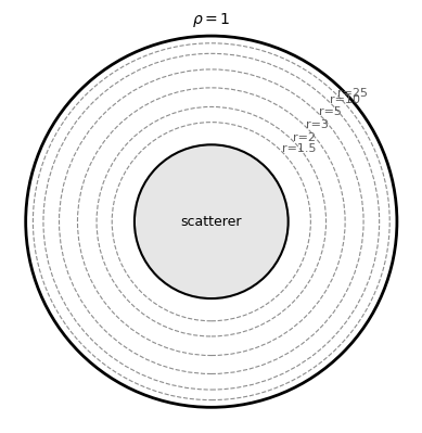
The coordinate diagram below shows the same accumulation using constant-\(r\) circles, each representing one physical radius. For the wave problem, however, a purely spatial compactification would squeeze infinitely many wavelengths into a finite layer as we discussed in Compactifying the Far Field. Hyperboloidal compactification adds the corresponding phase transformation, so outgoing waves become regular at the compactified boundary. The ideal boundary of the hyperbolic disk at \(\rho=1\) is then where the far-field pattern lives.

from ngsolve import *
from netgen.occ import *
from ngsolve.webgui import Draw
import numpy as np
from scipy.special import jv, hankel1
import matplotlib.pyplot as plt
from matplotlib.patches import Circle as MplCircle
from mpl_toolkits.axes_grid1.inset_locator import inset_axes
import ngsolve_special_functions as ng_sp
import time
notebook_start = time.perf_counter()

Poincaré radial coordinate used below

The compactification above is encoded in the conformal factor

\[ \Omega(\rho) = \frac{1-\rho^2}{2}, \qquad r = \frac{\rho}{\Omega} = \frac{2\rho}{1-\rho^2}. \]

The physical unit circle is therefore located at

\[ \rho_{\rm sc} = \sqrt{2}-1. \]

The outer boundary \(\rho=1\) represents infinity. In the finite-element solve below it’s named scri, following the standard notation for null infinity.

# Physical and compactified geometry
r_scatterer = 1.0
rho_outer = 1.0
rho_scatterer = np.sqrt(2.0) - 1.0

# Discretization
# Common circle-comparison target: order 8 and approximately 8,000 DOFs.
maxh = 0.140
order = 8

# Wavenumber and Fourier-Bessel truncation for the reference solution
k = 6.0
n_modes = 35

# Nominal physical mesh scale at the obstacle. Netgen's maxh is an upper bound.
dr_drho_scatterer = 2 * (1 + rho_scatterer**2) / (1 - rho_scatterer**2) ** 2
nominal_kh_over_p = k * maxh * dr_drho_scatterer / order

print(f"compactified scatterer radius: {rho_scatterer:.6f}")
print(f"ka = {k * r_scatterer:.1f}, nominal near-obstacle kh/p = {nominal_kh_over_p:.3f}")

compactified scatterer radius: 0.414214
ka = 6.0, nominal near-obstacle kh/p = 0.358

The following plot shows the compactified disk used for the computation. Each gray curve is a constant-\(r\) circle labelled by its physical radius. Their Euclidean coordinate spacing shrinks near rho = 1; the boundary itself remains infinitely far away in the hyperbolic metric.

def rho_from_physical_radius(r):
    return r / (np.sqrt(1 + r**2) + 1)

fig, ax = plt.subplots(figsize=(4.8, 4.8))
ax.add_patch(MplCircle((0, 0), rho_outer, fill=False, lw=2.0, color="black"))
ax.add_patch(MplCircle((0, 0), rho_scatterer, facecolor="0.90", edgecolor="black", lw=1.5))

for radius in [1.5, 2, 3, 5, 10, 25]:
    rho_radius = rho_from_physical_radius(radius)
    ax.add_patch(MplCircle((0, 0), rho_radius, fill=False, lw=0.8, ls="--", color="0.55"))
    ax.text(rho_radius / np.sqrt(2), rho_radius / np.sqrt(2), f"r={radius:g}", fontsize=8, color="0.35")

ax.text(0, 0, "scatterer", ha="center", va="center", fontsize=9)
ax.text(0, 1.04, r"$\rho=1$", ha="center", va="bottom", fontsize=10)
ax.set_aspect("equal")
ax.set_xlim(-1.08, 1.08)
ax.set_ylim(-1.08, 1.08)
ax.axis("off")
plt.show()

Geometry and hyperboloidal solve

For this compactification, the height function is

\[ h(r) = \sqrt{1+r^2} = \frac{1+\rho^2}{1-\rho^2}, \]

and its boost is

\[ H = \frac{dh}{dr} = \frac{2\rho}{1+\rho^2}. \]

The two-dimensional transformed unknown is given by

\[ U = \Omega^{1/2} e^{i k h} u. \]

def create_poincare_circle_geometry(rho_scatterer=rho_scatterer, rho_outer=rho_outer, draw=False):
    domain = Circle((0, 0), rho_outer).Face()
    domain.edges.name = "scri"
    domain.faces.name = "poincare"

    scatterer = Circle((0, 0), rho_scatterer).Face()
    scatterer.edges.name = "scatterer"

    annulus = domain - scatterer
    annulus.faces.name = "poincare"

    if draw:
        Draw(annulus)
    return OCCGeometry(annulus, dim=2)

geo = create_poincare_circle_geometry(draw=True)

def solve_poincare_circle(maxh=maxh, order=order, k=k):
    mesh = Mesh(create_poincare_circle_geometry(draw=False).GenerateMesh(maxh=maxh))
    mesh.Curve(order)

    fes = H1(mesh, order=order, complex=True, dirichlet=mesh.Boundaries("scatterer"))
    u, v = fes.TnT()

    rho = sqrt(x**2 + y**2)
    radial = CF((x, y))
    Q = OuterProduct(radial, radial) / rho**2
    P = Id(2) - Q

    Omega = (1 - rho**2) / 2
    DOmega = -rho
    L = Omega - rho * DOmega
    G = Omega**2 / L

    H = 2 * rho / (1 + rho**2)
    mu = 2 / (1 + rho**2)

    mass = mu * u * v * dx(bonus_intorder=6)
    transport = (
        -H / rho * u * InnerProduct(radial, grad(v)) * dx(bonus_intorder=6)
        + H / rho * v * InnerProduct(radial, grad(u)) * dx(bonus_intorder=6)
        + u * v * ds("scri")
    )
    stiffness = (
        -grad(u) * ((G * Q + L * P) * grad(v)) * dx(bonus_intorder=6)
        - Omega / L / (2 * rho) * DOmega * InnerProduct(grad(u), radial) * v * dx(bonus_intorder=6)
        - Omega / L / (2 * rho) * DOmega * InnerProduct(grad(v), radial) * u * dx(bonus_intorder=6)
        - 1 / L / 4 * DOmega**2 * u * v * dx(bonus_intorder=6)
    )

    A = BilinearForm(k**2 * mass + 1j * k * transport + stiffness).Assemble().mat
    Ainv = A.Inverse(freedofs=fes.FreeDofs())

    direction_dot_n = x / rho
    h_inner = np.sqrt(1 + r_scatterer**2)
    Omega_inner = rho_scatterer / r_scatterer
    boundary_data = -Omega_inner**(-0.5) * exp(1j * k * (r_scatterer * direction_dot_n - h_inner))

    gfu = GridFunction(fes)
    gfu.Set(boundary_data, definedon=mesh.Boundaries("scatterer"))

    residual = -A * gfu.vec
    gfu.vec.data += Ainv * residual
    return gfu

solve_start = time.perf_counter()
gfu = solve_poincare_circle()
solve_seconds = time.perf_counter() - solve_start
mesh = gfu.space.mesh
print(f"degrees of freedom: {gfu.space.ndof}")
print(f"mesh, assembly, and direct solve: {solve_seconds:.3f} s")

degrees of freedom: 8128
mesh, assembly, and direct solve: 0.248 s

Analytic far field

The common Fourier–Bessel reference is given in Common circle benchmark. With this Poincaré compactification and \(h(r)-r\to0\), this notebook extracts the numerical far field simply as

\[ U_{\infty,h}(\theta)=u_h(\rho=1,\theta). \]

def far_field_cf(k=k, N=n_modes):
    rho = sqrt(x**2 + y**2)
    nx = x / rho
    ny = y / rho

    cf = -ng_sp.jv(k, 0) / ng_sp.hankel1(k, 0)
    for n in range(1, N + 1):
        angular = (nx + 1j * ny) ** n + (nx - 1j * ny) ** n
        cf -= angular * ng_sp.jv(k, n) / ng_sp.hankel1(k, n)

    return np.sqrt(2 / (np.pi * k)) * np.exp(-1j * np.pi / 4) * cf


def far_field_pattern(thetas, k=k, N=n_modes):
    thetas = np.asarray(thetas, dtype=float)
    n = np.arange(-N, N + 1)
    coefficients = -jv(n, k) / hankel1(n, k)
    return np.sqrt(2 / (np.pi * k)) * np.exp(-1j * np.pi / 4) * (
        coefficients @ np.exp(1j * np.outer(n, thetas))
    )


def far_field_l2_error(gfu, reference_ff):
    mesh = gfu.space.mesh
    difference = gfu - reference_ff
    err_sq = Integrate(difference * Conj(difference), mesh, definedon=mesh.Boundaries("scri")).real
    norm_sq = Integrate(reference_ff * Conj(reference_ff), mesh, definedon=mesh.Boundaries("scri")).real
    return np.sqrt(err_sq / norm_sq)


def sample_far_field(gfu, thetas, eps=1e-8):
    sample_radius = 1 - eps
    return np.array(
        [gfu(sample_radius * np.cos(theta), sample_radius * np.sin(theta)) for theta in thetas],
        dtype=complex,
    )

reference_start = time.perf_counter()
reference_far_field = far_field_cf()
far_field_rel_error = far_field_l2_error(gfu, reference_far_field)
reference_seconds = time.perf_counter() - reference_start
print(f"relative far-field L2 error at scri: {far_field_rel_error:.3e}")
print(f"analytic reference evaluation: {reference_seconds:.3f} s")

relative far-field L2 error at scri: 5.615e-08
analytic reference evaluation: 0.090 s

Far-field angular distribution

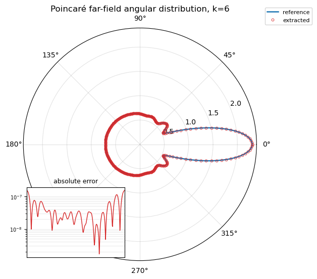
The polar plot compares the extracted far field with the analytic far-field pattern. The inset shows the absolute error as a function of angle.

thetas = np.linspace(0, 2 * np.pi, 361, endpoint=True)
ff_num = sample_far_field(gfu, thetas)
ff_ref = far_field_pattern(thetas)
absolute_error = np.abs(ff_num - ff_ref)

fig = plt.figure(figsize=(6, 6))
ax = fig.add_subplot(111, projection="polar")

ax.plot(thetas, np.abs(ff_ref), color="C0", lw=1.8, label="reference")
ax.plot(
    thetas,
    np.abs(ff_num),
    linestyle="None",
    marker="o",
    markerfacecolor="none",
    markersize=3.5,
    markeredgewidth=0.6,
    color="C3",
    label="extracted",
)
ax.set_title(f"Poincaré far-field angular distribution, k={k:g}", pad=24)
ax.grid(True, alpha=0.35)
ax.legend(loc="upper right", bbox_to_anchor=(1.25, 1.10), fontsize=8)

axins = inset_axes(ax, width="42%", height="30%", loc="lower left")
axins.semilogy(thetas, np.maximum(absolute_error, 1e-16), color="C3", lw=1)
axins.set_title("absolute error", fontsize=9)
axins.set_xlim(0, 2 * np.pi)
axins.set_xticks([])
axins.tick_params(axis="y", labelsize=7)
axins.grid(True, which="both", alpha=0.25)

plt.show()

Compactified solution

The plotted field is the hyperboloidal unknown u, not the physical scattered field U. Its finite trace at the outer boundary is the far-field pattern.

Draw(gfu, mesh, "Poincaré compactified scattered field", min=-1, max=1)
print(f"notebook compute time after imports: {time.perf_counter() - notebook_start:.3f} s")

notebook compute time after imports: 0.748 s

Remarks

• The whole exterior of the centered disk is represented in the Poincaré disk.

• The outer circle is not an artificial boundary; it’s the compactified representation of infinity, also referred to as the ideal boundary of hyperbolic geometry. In the spacetime picture, this boundary corresponds to a cut of future null infinity.

• The construction links three viewpoints: the hyperboloid model of hyperbolic geometry, conformal compactification of infinity, and the outgoing radiation condition for the Helmholtz equation.