Frequency Domain: Sound-Soft Circle

Next, we attach a hyperboloidal layer representing the exterior domain for the Common circle benchmark. Unlike the previous global compactifications, the layer uses standard coordinates near the obstacle and transforms only the far field. Its outer boundary represents infinity as before.

from ngsolve import *
from netgen.occ import *
from ngsolve.webgui import Draw
import numpy as np
from scipy.special import jv, hankel1
import matplotlib.pyplot as plt
from mpl_toolkits.axes_grid1.inset_locator import inset_axes
import ngsolve_special_functions as ng_sp
import time
notebook_start = time.perf_counter()

Parameters

The obstacle is a centered unit circle so this layer calculation can be compared directly with the characteristic and Poincaré notebooks. This implementation also allows experiments with shifted circles by changing the parameter MScat. The computational mesh has two regions:

• an inner physical region, where the coordinates are unchanged;

• an outer compactifying layer, where the coordinate transformation moves infinity to the finite radius Rout.

All three circle benchmarks use eighth-order elements and are tuned to approximately 8,000 degrees of freedom to make their errors comparable at a fixed computational budget.

# Geometry parameters
Rout = 2.0
RScat = 1.0
MScat = (0.0, 0.0)
R = 1.5

# Discretization parameters
# Common circle-comparison target: order 8 and approximately 8,000 DOFs.
maxh = 0.288
order = 8

# Problem parameter
k = 6.0

# Here maxh is already a physical mesh scale in the unchanged inner region.
nominal_kh_over_p = k * maxh / order

Geometry

The finite computational domain is a disk of radius Rout with a circular hole. The interface radius R separates the physical region from the compactifying layer.

def create_circle_geometry(Rout=Rout, RScat=RScat, MScat=MScat, R=R, draw=False):
    domain = Circle((0, 0), Rout).Face()
    domain.edges.name = "outer"
    domain.faces.name = "outer"

    scatterer = Circle(MScat, RScat).Face()
    scatterer.edges.name = "scatterer"

    inner = Circle((0, 0), R).Face()
    inner.edges.name = "interface"
    inner.faces.name = "inner"

    pieces = Glue([domain - inner, inner - scatterer])
    if draw:
        Draw(pieces)
    return OCCGeometry(pieces, dim=2)

geo = create_circle_geometry(draw=True)

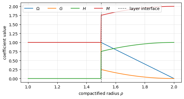
Layer coefficient profiles

The profiles below connect the geometry to the weak form before assembly. The transformation is the identity for \(\rho\le R\). Across the fitted interface, \(\Omega\) is continuous. In the layer, \(G\) tends to zero, \(H=1-G\) tends to one, and \(M=(1-H^2)/G=1+H\) remains bounded.

rho_profile = np.linspace(RScat, Rout, 500)
in_layer = rho_profile > R
Omega_profile = np.where(in_layer, (Rout - rho_profile) / (Rout - R), 1.0)
L_profile = np.where(in_layer, Rout / (Rout - R), 1.0)
G_profile = Omega_profile**2 / L_profile
H_profile = np.where(in_layer, 1 - G_profile, 0.0)
M_profile = np.where(in_layer, 1 + H_profile, 1.0)

fig, ax = plt.subplots(figsize=(7, 3.5))
for values, label in [(Omega_profile, r"$\Omega$"), (G_profile, r"$G$"),
                      (H_profile, r"$H$"), (M_profile, r"$M$")]:
    ax.plot(rho_profile, values, label=label)
ax.axvline(R, color="0.3", ls="--", lw=1, label="layer interface")
ax.set(xlabel=r"compactified radius $\rho$", ylabel="coefficient value")
ax.grid(True, alpha=0.3)
ax.legend(ncol=5)
plt.show()

Hyperboloidal FEM solve

The compactification is encoded by the conformal factor

\[ \Omega = \frac{R_{\rm out} - \rho}{R_{\rm out} - R} \]

in the outer layer and \(\Omega=1\) in the inner region. The coefficient functions G, L, H, and M enter the transformed Helmholtz operator. The choice H = 1 - G is the characteristic-preserving boost used in the paper.

def solve_circle_hyperboloidal(maxh=maxh, order=order, k=k):
    geo = create_circle_geometry(draw=False)
    mesh = Mesh(geo.GenerateMesh(maxh=maxh))
    mesh.Curve(order)

    fes = H1(mesh, order=order, complex=True, dirichlet=mesh.Boundaries("scatterer"))
    w, v = fes.TnT()

    rho = sqrt(x**2 + y**2)
    Omega = mesh.MaterialCF({"outer": (Rout - rho) / (Rout - R)}, default=1)
    DOmega = Omega.Diff(rho)
    L = Omega - rho * DOmega
    G = Omega**2 / L

    H = mesh.MaterialCF({"outer": 1 - G}, default=0)
    M = 1 + H  # (1-H**2)/G for H=1-G

    radial = CF((x, y))
    Q = OuterProduct(radial, radial) / rho**2
    P = Id(2) - Q

    mass = M * w * v * dx(bonus_intorder=4)

    transport = (
        -H / rho * w * InnerProduct(radial, grad(v)) * dx(bonus_intorder=4)
        + H / rho * v * InnerProduct(radial, grad(w)) * dx(bonus_intorder=4)
        + v * w * ds("outer")
    )

    stiffness = (
        -grad(w) * ((G * Q + L * P) * grad(v)) * dx(bonus_intorder=4)
        - Omega / L / (2 * rho) * DOmega * InnerProduct(grad(w), radial) * v * dx(bonus_intorder=4)
        - Omega / L / (2 * rho) * DOmega * InnerProduct(grad(v), radial) * w * dx(bonus_intorder=4)
        - 1 / L / 4 * DOmega**2 * w * v * dx(bonus_intorder=4)
    )

    A = BilinearForm(k**2 * mass + 1j * k * transport + stiffness).Assemble().mat
    Ainv = A.Inverse(freedofs=fes.FreeDofs())

    boundary_data = -exp(1j * k * x)
    gfu = GridFunction(fes)
    gfu.Set(boundary_data, definedon=mesh.Boundaries("scatterer"))

    residual = -A * gfu.vec
    gfu.vec.data += Ainv * residual
    return gfu

solve_start = time.perf_counter()
gfu = solve_circle_hyperboloidal()
solve_seconds = time.perf_counter() - solve_start
print(f"degrees of freedom: {gfu.space.ndof}")
print(f"ka = {k * RScat:.1f}, nominal inner-region kh/p = {nominal_kh_over_p:.3f}")
print(f"mesh, assembly, and direct solve: {solve_seconds:.3f} s")

degrees of freedom: 8712
ka = 6.0, nominal inner-region kh/p = 0.216
mesh, assembly, and direct solve: 0.231 s

Analytic reference solution

The explicit solution in the form of a Fourier–Bessel series is given in Common circle benchmark. We use ngsolve_special_functions to represent it as an NGSolve coefficient function.

The near-field error below is measured only on the inner physical region, where the compactification is the identity and the numerical unknown agrees with the physical scattered field. Constructing and projecting the explicit solution throughout the compactified layer is substantially more expensive than assembling and solving the finite-element problem, so we do not perform that full-domain projection here.

def reference_solution_cf(k=k, N=35, MScat=MScat, xphys=x, yphys=y):
    xm = xphys - MScat[0]
    ym = yphys - MScat[1]
    r = sqrt(xm**2 + ym**2)

    cf = -ng_sp.jv(k, 0) / ng_sp.hankel1(k, 0) * ng_sp.hankel1(k * r, 0)
    for n in range(1, N + 1):
        angular = ((xm + 1j * ym) / r) ** n + ((xm - 1j * ym) / r) ** n
        coeff = -ng_sp.jv(k, n) / ng_sp.hankel1(k, n) * (1j**n) * ng_sp.hankel1(k * r, n)
        cf += angular * coeff

    return np.exp(1j * k * MScat[0]) * cf


def far_field_cf(k=k, N=35, MScat=MScat):
    rho = sqrt(x**2 + y**2)
    nx = x / rho
    ny = y / rho

    cf = -ng_sp.jv(k, 0) / ng_sp.hankel1(k, 0)
    for n in range(1, N + 1):
        angular = (nx + 1j * ny) ** n + (nx - 1j * ny) ** n
        cf -= angular * ng_sp.jv(k, n) / ng_sp.hankel1(k, n)

    shift = exp(1j * k * (MScat[0] - MScat[0] * nx - MScat[1] * ny))
    return np.sqrt(2 / (np.pi * k)) * np.exp(-1j * np.pi / 4) * shift * cf


def far_field_pattern(thetas, k=k, N=35, MScat=MScat):
    thetas = np.asarray(thetas, dtype=float)
    n = np.arange(-N, N + 1)
    centered = (-jv(n, k) / hankel1(n, k)) @ np.exp(1j * np.outer(n, thetas))
    shift = np.exp(1j * k * (MScat[0] - MScat[0] * np.cos(thetas) - MScat[1] * np.sin(thetas)))
    return np.sqrt(2 / (np.pi * k)) * np.exp(-1j * np.pi / 4) * shift * centered


def extracted_far_field_cf(gfu, k=k):
    return np.sqrt(Rout) * np.exp(-1j * k * Rout) * gfu


def far_field_l2_error(gfu, reference_ff):
    mesh = gfu.space.mesh
    numerical_ff = extracted_far_field_cf(gfu)
    difference = numerical_ff - reference_ff
    err_sq = Integrate(difference * Conj(difference), mesh, definedon=mesh.Boundaries("outer")).real
    norm_sq = Integrate(reference_ff * Conj(reference_ff), mesh, definedon=mesh.Boundaries("outer")).real
    return np.sqrt(err_sq / norm_sq), numerical_ff


def sample_extracted_far_field(gfu, thetas, eps=1e-8):
    sample_radius = (1 - eps) * Rout
    scale = np.sqrt(Rout) * np.exp(-1j * k * Rout)
    return scale * np.array(
        [gfu(sample_radius * np.cos(theta), sample_radius * np.sin(theta)) for theta in thetas],
        dtype=complex,
    )


def l2_error_projected(gfu, ref, definedon):
    u, v = gfu.space.TnT()
    mass = BilinearForm(u * v * dx(definedon), check_unused=False).Assemble().mat

    gfref = GridFunction(gfu.space)
    gfref.Set(ref, definedon=definedon)

    error = gfu.vec.CreateVector()
    error.data = gfref.vec - gfu.vec

    err_norm = sqrt(error.InnerProduct(mass * error).real)
    ref_norm = sqrt(gfref.vec.InnerProduct(mass * gfref.vec).real)
    return err_norm, ref_norm

reference_start = time.perf_counter()
reference_inner = reference_solution_cf()
reference_far_field = far_field_cf()
far_field_rel_error, numerical_far_field = far_field_l2_error(gfu, reference_far_field)

err, ref_norm = l2_error_projected(gfu, reference_inner, gfu.space.mesh.Materials("inner"))
reference_seconds = time.perf_counter() - reference_start
print(f"relative L2 error on inner region: {err / ref_norm:.3e}")
print(f"relative far-field L2 error at scri: {far_field_rel_error:.3e}")
print(f"explicit Fourier-Bessel reference evaluation: {reference_seconds:.3f} s")
print(f"reference / solve time ratio: {reference_seconds / solve_seconds:.1f}x")

relative L2 error on inner region: 4.403e-08
relative far-field L2 error at scri: 3.176e-08
explicit Fourier-Bessel reference evaluation: 1.493 s
reference / solve time ratio: 6.5x

Far-field comparison

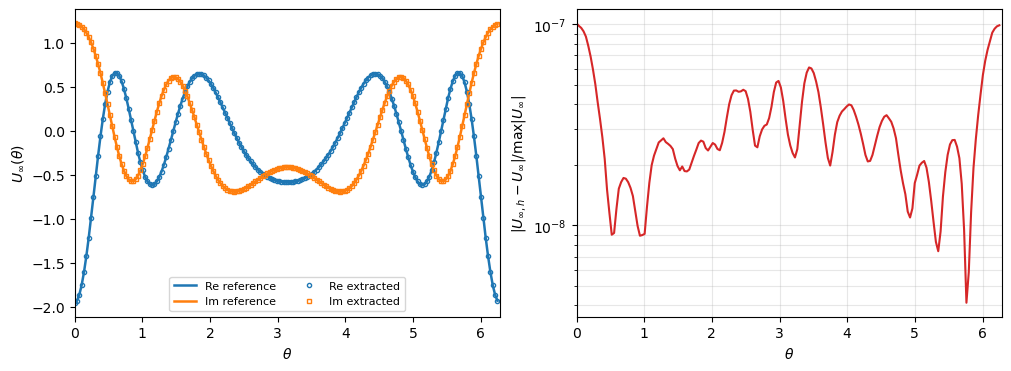
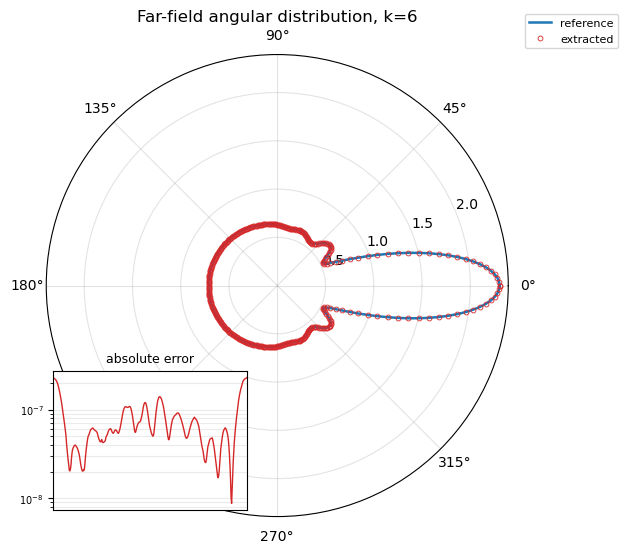
At the compactified outer boundary, the trace of the hyperboloidal unknown gives the far-field pattern up to a constant phase and amplitude factor. For this layer the extracted numerical far field is

\[ U_{\infty,h}(\theta) = \sqrt{R_{\rm out}} e^{-i k R_{\rm out}} u_h(R_{\rm out},\theta). \]

We compare this boundary trace with the analytic far-field series for the disk. The first figure compares the complex-valued far field as a function of angle. The second figure shows the angular distribution \(|U_\infty(\theta)|\) in polar form.

thetas = np.linspace(0, 2 * np.pi, 181, endpoint=False)
ff_num = sample_extracted_far_field(gfu, thetas)
ff_ref = far_field_pattern(thetas)
normalized_pointwise_error = np.abs(ff_num - ff_ref) / np.max(np.abs(ff_ref))

fig, (ax_field, ax_error) = plt.subplots(1, 2, figsize=(10, 3.6), constrained_layout=True)

ax_field.plot(thetas, ff_ref.real, color="C0", lw=1.8, label="Re reference")
ax_field.plot(thetas, ff_ref.imag, color="C1", lw=1.8, label="Im reference")
ax_field.plot(thetas, ff_num.real, "o", color="C0", ms=3, mfc="none", label="Re extracted")
ax_field.plot(thetas, ff_num.imag, "s", color="C1", ms=3, mfc="none", label="Im extracted")
ax_field.set_xlabel(r"$\theta$")
ax_field.set_ylabel(r"$U_\infty(\theta)$")
ax_field.set_xlim(0, 2 * np.pi)
ax_field.legend(ncol=2, fontsize=8)

ax_error.semilogy(thetas, np.maximum(normalized_pointwise_error, 1e-16), color="C3")
ax_error.set_xlabel(r"$\theta$")
ax_error.set_ylabel(r"$|U_{\infty,h}-U_\infty| / \max|U_\infty|$")
ax_error.set_xlim(0, 2 * np.pi)
ax_error.grid(True, which="both", alpha=0.3)

plt.show()

thetas_distribution = np.linspace(0, 2 * np.pi, 361, endpoint=True)
ff_num_distribution = sample_extracted_far_field(gfu, thetas_distribution)
ff_ref_distribution = far_field_pattern(thetas_distribution)
absolute_error = np.abs(ff_num_distribution - ff_ref_distribution)

fig = plt.figure(figsize=(6, 6))
ax = fig.add_subplot(111, projection="polar")

ax.plot(thetas_distribution, np.abs(ff_ref_distribution), color="C0", lw=1.8, label="reference")
ax.plot(
    thetas_distribution,
    np.abs(ff_num_distribution),
    linestyle="None",
    marker="o",
    markerfacecolor="none",
    markersize=3.5,
    markeredgewidth=0.6,
    color="C3",
    label="extracted",
)
ax.set_title(f"Far-field angular distribution, k={k:g}", pad=24)
ax.grid(True, alpha=0.35)
ax.legend(loc="upper right", bbox_to_anchor=(1.25, 1.10), fontsize=8)

axins = inset_axes(ax, width="42%", height="30%", loc="lower left")
axins.semilogy(thetas_distribution, np.maximum(absolute_error, 1e-16), color="C3", lw=1)
axins.set_title("absolute error", fontsize=9)
axins.set_xlim(0, 2 * np.pi)
axins.set_xticks([])
axins.tick_params(axis="y", labelsize=7)
axins.grid(True, which="both", alpha=0.25)

plt.show()

Visualization

The plot below shows the computed hyperboloidal unknown.

Draw(gfu, gfu.space.mesh, "hyperboloidal scattered field", min=-1, max=1)
print(f"notebook compute time after imports: {time.perf_counter() - notebook_start:.3f} s")

notebook compute time after imports: 2.602 s

Remarks

• The inner boundary condition is imposed as a Dirichlet condition for the scattered field. Since the transformations are restricted to an outer layer, the inner boundary condition is unchanged.

• The outer boundary term in transport is part of the transformed outgoing radiation condition at compactified infinity.

This is the basic pattern used in the more complicated trapping-square example and extends analogously to radial three-dimensional geometries.