Time Domain: Trapping Square with Discontinuous Galerkin

We solve the same driven trapping-square problem once more, now with discontinuous Galerkin elements. This is not to compare the speed or accuracy of DG and conforming elements. DG is interesting here because it exposes face terms. In particular, the lower-order derivatives from the conformal rescaling and the mixed time-space term must be coupled consistently across element faces.

The geometry, layer, source frequency, time step, and Newmark method are the same as before. We use a coarser DG discretization and a shorter evolution to keep the example quick. The spatial operator uses symmetric interior penalty, the mixed term uses a skew face coupling, and the sound-soft wall is imposed weakly. As before, the outer boundary is null infinity and needs no artificial boundary condition.

from ngsolve import *
from netgen.occ import *
from ngsolve.webgui import Draw
import matplotlib.pyplot as plt
import numpy as np
import time

notebook_start = time.perf_counter()

Where DG needs extra care

The compactified weak equation has the semidiscrete form

\[ M\ddot u+C\dot u+Ku=f. \]

To see the extra face terms, let \(X=(x,y)\), \(\rho=|X|\), \(Q=XX^T/\rho^2\), \(P=I-Q\), and \(A=GQ+LP\). We also define the regular vector

\[ g=\frac{\Omega\Omega'}{2L\rho}X. \]

The spatial volume form can be written as

\[ K(u,v)=\int_{\mathcal D} \left[\nabla u\cdot A\nabla v+g\cdot\nabla u\,v+g\cdot\nabla v\,u+\frac{(\Omega')^2}{4L}uv\right]dx. \]

The first three terms belong together: they come from the factored conformal derivative. The corresponding flux is therefore not just \(A\nabla u\), but

\[ \mathcal F(u)=A\nabla u+g u. \]

This is relevant at the layer interface, where \(g\) changes. If we used only \(A\nabla u\) in the DG face terms, we would discretize a different global operator.

The mixed time-space term has a different structure. With \(b=HX/\rho\),

\[ C(u,v)=\int_{\mathcal D}\left[v\,b\cdot\nabla u-u\,b\cdot\nabla v\right]dx +\int_{\mathscr I^+}uv\,ds. \]

The two volume terms form a skew pair. In a conforming method their face contributions cancel automatically. DG has two independent traces, so we must restore that coupling explicitly. Once this is done, the only quadratic contribution from \(C\) is the physical outflow through null infinity.

# Geometry
Rout = 2.0
RScat = 1.0
DScat = 0.1
DHole = 0.2
R = 1.5
xOffset = 0.5

# DG discretization
maxh = 0.20
order = 3
penalty = 8.0

# Time integration and source
dt = 2e-2
beta = 1 / 4
gamma = 1 / 2
drive_frequency = 10.8
drive_until = 3.0
t_end = 6.0
source_amplitude = 100.0

def create_trapping_geometry(draw=False):
    domain = Circle((0, 0), Rout).Face()
    domain.edges.name = "outer"
    domain.faces.name = "outer"

    inner = Circle((0, 0), R).Face()
    inner.edges.name = "interface"
    inner.faces.name = "inner"

    wall = (
        MoveTo(-RScat / 2 + xOffset, -RScat / 2).Rectangle(RScat, RScat).Face()
        - MoveTo(-RScat / 2 + DScat / 2 + xOffset, -RScat / 2 + DScat / 2)
          .Rectangle(RScat - DScat, RScat - DScat).Face()
        - MoveTo(-RScat / 2 - DScat + xOffset, -DHole / 2)
          .Rectangle(2 * DScat, DHole).Face()
    )
    wall.edges.name = "scatterer"

    cavity = (
        MoveTo(-RScat / 2 + xOffset, -RScat / 2).Rectangle(RScat, RScat).Face()
        - wall
    )
    cavity.faces.name = "cavity"

    pieces = Glue([domain - inner, inner - cavity - wall, cavity])
    if draw:
        Draw(pieces)
    return OCCGeometry(pieces, dim=2)


mesh = Mesh(create_trapping_geometry().GenerateMesh(maxh=maxh))
mesh.Curve(order)
fes = L2(mesh, order=order, dgjumps=True)
print(f"DG degrees of freedom: {fes.ndof}")
print(f"omega L = {drive_frequency * RScat:.1f}, nominal physical-region omega h/p = {drive_frequency * maxh / order:.3f}")

DG degrees of freedom: 7450
omega L = 10.8, nominal physical-region omega h/p = 0.720

Spatial flux and penalty

On an interior face \(F\), write \([u]=u^- -u^+\) and use braces for an average. The consistency terms are

\[ -\int_F\{\mathcal F(u)\cdot n\}[v],ds -\int_F\{\mathcal F(v)\cdot n\}[u],ds. \]

We add the usual penalty proportional to \((p+1)^2(n^TAn)/h\). The important choice is to use the full flux \(\mathcal F=A\nabla+g\), including its lower-order part. This keeps the face terms consistent with the continuous operator.

We use the same flux to impose the sound-soft wall weakly. At \(\mathscr I^+\) the radial diffusivity vanishes, so there is no SIPG boundary condition to add.

def assemble_dg_forms(mesh, fes):
    u, v = fes.TnT()
    rho = sqrt(x**2 + y**2)
    radial = CF((x, y))

    Omega = mesh.MaterialCF({"outer": (Rout - rho) / (Rout - R)}, default=1)
    DOmega = Omega.Diff(rho)
    L = Omega - rho * DOmega
    G = Omega**2 / L
    H = mesh.MaterialCF({"outer": 1 - G}, default=0)
    mass_weight = 1 + H  # (1-H**2)/G for H=1-G

    Q = OuterProduct(radial, radial) / rho**2
    P = Id(2) - Q
    A = G * Q + L * P
    conformal_vector = Omega / L / (2 * rho) * DOmega * radial

    normal = specialcf.normal(mesh.dim)
    mesh_size = specialcf.mesh_size
    jump_u = u - u.Other()
    jump_v = v - v.Other()

    # The lower-order conformal term belongs in the consistency flux.
    flux_vector_u = A * grad(u) + conformal_vector * u
    flux_vector_v = A * grad(v) + conformal_vector * v
    flux_vector_u_other = A.Other() * grad(u.Other()) + conformal_vector.Other() * u.Other()
    flux_vector_v_other = A.Other() * grad(v.Other()) + conformal_vector.Other() * v.Other()
    average_flux_u = 0.5 * (flux_vector_u + flux_vector_u_other)
    average_flux_v = 0.5 * (flux_vector_v + flux_vector_v_other)

    normal_diffusion = InnerProduct(normal, A * normal)
    normal_diffusion_other = InnerProduct(normal, A.Other() * normal)
    average_normal_diffusion = 0.5 * (normal_diffusion + normal_diffusion_other)
    average_h = 0.5 * (mesh_size + mesh_size.Other())
    sigma = penalty * (order + 1) ** 2 * average_normal_diffusion / average_h

    stiffness_volume = (
        InnerProduct(grad(u), A * grad(v))
        + InnerProduct(conformal_vector, grad(u)) * v
        + InnerProduct(conformal_vector, grad(v)) * u
        + DOmega**2 / (4 * L) * u * v
    ) * dx
    stiffness_faces = (
        -InnerProduct(average_flux_u, normal) * jump_v
        -InnerProduct(average_flux_v, normal) * jump_u
        + sigma * jump_u * jump_v
    ) * dx(skeleton=True)

    # Weak homogeneous Dirichlet condition on the sound-soft wall.
    boundary_sigma = penalty * (order + 1) ** 2 * normal_diffusion / mesh_size
    stiffness_wall = (
        -InnerProduct(flux_vector_u, normal) * v
        -InnerProduct(flux_vector_v, normal) * u
        + boundary_sigma * u * v
    ) * ds("scatterer", skeleton=True)

    # Skew volume-plus-skeleton form for the mixed time-space term.
    transport_vector = H / rho * radial
    average_transport = 0.5 * (transport_vector + transport_vector.Other())
    normal_transport = InnerProduct(average_transport, normal)
    transport = (
        -u * InnerProduct(transport_vector, grad(v)) * dx
        + v * InnerProduct(transport_vector, grad(u)) * dx
        + normal_transport * (u.Other() * v - u * v.Other()) * dx(skeleton=True)
        + u * v * ds("outer", skeleton=True)
    )

    mass = mass_weight * u * v * dx
    stiffness = stiffness_volume + stiffness_faces + stiffness_wall
    return mass, transport, stiffness


mass_form, transport_form, stiffness_form = assemble_dg_forms(mesh, fes)

The mixed skeleton term

For a conforming function the two traces agree, so the interior-face term in \(C_h\) disappears. For a DG function it supplies the coupling produced when \(-u\,b\cdot\nabla v\) is integrated by parts on each element. The face term is skew: exchanging trial and test functions changes its sign. The volume and face contributions therefore make no quadratic contribution, leaving only

\[ C_h(w,w)=\int_{\mathscr I^+}w^2\,ds. \]

This is the outgoing energy flux. If we omit the skeleton term, the check \(C_h(w,w)\) may still look correct because the elementwise volume pair is already skew. What is lost is the transport between elements. We must test different trial and test traces to see the inconsistency; an energy check alone is not enough.

The fitted interface between the physical region and the layer needs no special treatment. It is an ordinary DG face, evaluated with the coefficients and traces from both sides.

Newmark evolution

Time stepping is the same as in the conforming notebook. With \(\beta=1/4\) and \(\gamma=1/2\), every step reuses

\[ S^{-1}=\left(M+\gamma\Delta t C+\beta\Delta t^2K\right)^{-1}. \]

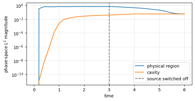
The predictor form needs one K product, one C product, and one application of \(S^{-1}\) per step. The initial state and the sinusoidal load at \(t=0\) vanish, so no separate mass inverse is needed. We sample the diagnostic every \(0.2\) time units and save an animation frame every \(0.5\) time units. These choices affect only the output, not the Newmark evolution.

assembly_start = time.perf_counter()
C = BilinearForm(transport_form).Assemble().mat
K = BilinearForm(stiffness_form).Assemble().mat
Sinv = BilinearForm(
    mass_form + gamma * dt * transport_form + beta * dt**2 * stiffness_form
).Assemble().mat.Inverse()
assembly_seconds = time.perf_counter() - assembly_start

u, v = fes.TnT()
outer_flux_matrix = BilinearForm(
    u * v * ds("outer", skeleton=True),
    check_unused=False,
).Assemble().mat
probe = GridFunction(fes)
probe.vec.FV().NumPy()[:] = np.random.default_rng(7).standard_normal(fes.ndof)
mixed_quadratic = probe.vec.InnerProduct(C * probe.vec).real
outflow_quadratic = probe.vec.InnerProduct(outer_flux_matrix * probe.vec).real
mixed_identity_residual = abs(mixed_quadratic - outflow_quadratic) / abs(outflow_quadratic)

source_profile = exp(-30 * ((x + 0.8) ** 2 + (y + 0.8) ** 2))
force = LinearForm(
    source_amplitude * source_profile * v * dx("inner|cavity")
).Assemble().vec
effective_force = Sinv * force

solution = GridFunction(fes, name="u_dg")
velocity = GridFunction(fes, name="ut_dg")
acceleration = GridFunction(fes, name="utt_dg")  # zero for the present initial data
old_acceleration = acceleration.vec.CreateVector()
predicted_solution = acceleration.vec.CreateVector()
predicted_velocity = acceleration.vec.CreateVector()
acceleration_rhs = acceleration.vec.CreateVector()

physical_mass = BilinearForm(
    u * v * dx("inner|cavity"), check_unused=False
).Assemble().mat
cavity_mass = BilinearForm(
    u * v * dx("cavity"), check_unused=False
).Assemble().mat

sample_times = []
physical_magnitudes = []
cavity_magnitudes = []
animation = GridFunction(fes, multidim=0, name="u_dg_history")
diagnostic_stride = max(1, int(round(0.2 / dt)))
frame_stride = max(1, int(round(0.5 / dt)))
evolution_start = time.perf_counter()
nsteps = int(round(t_end / dt))

for step in range(nsteps):
    t = step * dt
    if step % diagnostic_stride == 0:
        physical_q = solution.vec.InnerProduct(physical_mass * solution.vec).real
        physical_v = velocity.vec.InnerProduct(physical_mass * velocity.vec).real
        cavity_q = solution.vec.InnerProduct(cavity_mass * solution.vec).real
        cavity_v = velocity.vec.InnerProduct(cavity_mass * velocity.vec).real
        sample_times.append(t)
        physical_magnitudes.append(np.sqrt(max(0, physical_q + physical_v / drive_frequency**2)))
        cavity_magnitudes.append(np.sqrt(max(0, cavity_q + cavity_v / drive_frequency**2)))
    if step % frame_stride == 0:
        animation.AddMultiDimComponent(solution.vec)

    old_acceleration.data = acceleration.vec
    predicted_solution.data = solution.vec
    predicted_solution.data += dt * velocity.vec
    predicted_solution.data += (0.5 - beta) * dt**2 * old_acceleration
    predicted_velocity.data = velocity.vec
    predicted_velocity.data += (1 - gamma) * dt * old_acceleration

    acceleration_rhs.data = -K * predicted_solution
    acceleration_rhs.data += -C * predicted_velocity
    acceleration.vec.data = Sinv * acceleration_rhs
    if t + dt < drive_until:
        acceleration.vec.data += (
            np.sin(drive_frequency * (t + dt)) * effective_force
        )

    solution.vec.data = predicted_solution
    solution.vec.data += beta * dt**2 * acceleration.vec
    velocity.vec.data = predicted_velocity
    velocity.vec.data += gamma * dt * acceleration.vec

physical_q = solution.vec.InnerProduct(physical_mass * solution.vec).real
physical_v = velocity.vec.InnerProduct(physical_mass * velocity.vec).real
cavity_q = solution.vec.InnerProduct(cavity_mass * solution.vec).real
cavity_v = velocity.vec.InnerProduct(cavity_mass * velocity.vec).real
sample_times.append(t_end)
physical_magnitudes.append(np.sqrt(max(0, physical_q + physical_v / drive_frequency**2)))
cavity_magnitudes.append(np.sqrt(max(0, cavity_q + cavity_v / drive_frequency**2)))
animation.AddMultiDimComponent(solution.vec)  # include the state at t=t_end
evolution_seconds = time.perf_counter() - evolution_start
sample_times = np.asarray(sample_times)
physical_magnitudes = np.asarray(physical_magnitudes)
cavity_magnitudes = np.asarray(cavity_magnitudes)
print(f"mixed-form outflow identity residual: {mixed_identity_residual:.3e}")
print(f"matrix assembly and factorization: {assembly_seconds:.3f} s")
print(f"Newmark evolution ({nsteps} steps): {evolution_seconds:.3f} s")

mixed-form outflow identity residual: 4.507e-16
matrix assembly and factorization: 1.300 s
Newmark evolution (300 steps): 2.588 s

Draw(
    animation, mesh, "DG compactified time evolution",
    min=-0.1, max=0.1, animate=True,
)

fig, ax = plt.subplots(figsize=(7, 3.5))
ax.semilogy(sample_times, physical_magnitudes, label="physical region")
ax.semilogy(sample_times, cavity_magnitudes, label="cavity")
ax.axvline(drive_until, color="0.4", ls="--", label="source switched off")
ax.set(xlabel="time", ylabel="phase-space $L^2$ magnitude")
ax.grid(True, which="both", alpha=0.3)
ax.legend()
plt.show()
print(f"notebook compute time after imports: {time.perf_counter() - notebook_start:.3f} s")

notebook compute time after imports: 4.337 s

Interpretation

Inside the layer interface, the animated DG unknown is the original scalar field. It remains regular through the layer and at null infinity. After the source is switched off, radiation leaves the domain while part of the wave continues to ring in the cavity as before. The calculation shows that both the fitted layer interface and compactified infinity fit naturally into DG once the correct flux structure is retained.

Here we use a central, energy-balanced treatment of the mixed operator and SIPG stabilization for spatial jumps. Upwind or Rusanov dissipation fits more naturally after rewriting the wave equation as a first-order characteristic system. The first- and second-order formulations are related, but their fluxes should not be combined without rederiving the discrete operator.

The main lesson from this example is to keep conservative and skew pairs together when constructing the DG form. If variable-coefficient derivatives are expanded into unrelated lower-order terms, the code may look reasonable on each element but would be missing the correct coupling between elements.